Tutorial 3: SciPy
This sections shows several examples how to use module SciPy. See module homepage for more tutorials, reference manual.
Integration
import scipy.integrate as sc
import numpy as np

# 1-D
sc.quad(lambda x :np.exp(-x**2), -np.inf, np.inf)[0]
1.77245385091

# 2-D
sc.dblquad(lambda x, y: x*y, 0, 2, lambda x: 0, lambda x: 2)[0]
4.0
Interpolation
import scipy.interpolate as sc
import matplotlib.pyplot as plt

# 1-D
x = np.linspace(0, 10, 11)
y = np.sin(x)
x2 = np.linspace(0, 10, 100)
y2 = sc.interp1d(x, y)

plt.figure()
plt.plot(x, y, 'o')
plt.plot(x2, y2(x2))
plt.show()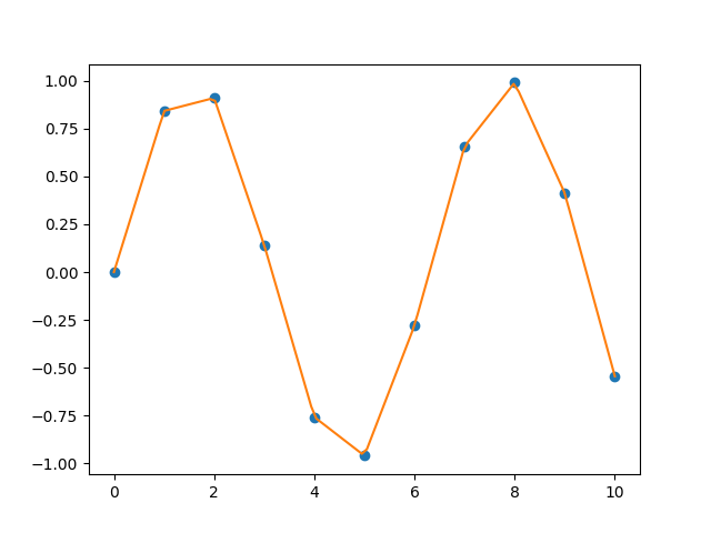
Fourier transform
import scipy.fftpack as sc

# 2 waves
N = 600
T = 1.0 / 800.0
x = np.linspace(0.0, N*T, N)
y = np.sin(50.0 * 2.0*np.pi*x) + 0.5*np.sin(80.0 * 2.0*np.pi*x)
xf = np.linspace(0.0, 1.0/(2.0*T), N//2)
yf = sc.fft(y)

plt.figure()
plt.plot(xf, 2.0/N * np.abs(yf[0:N//2]))
plt.show()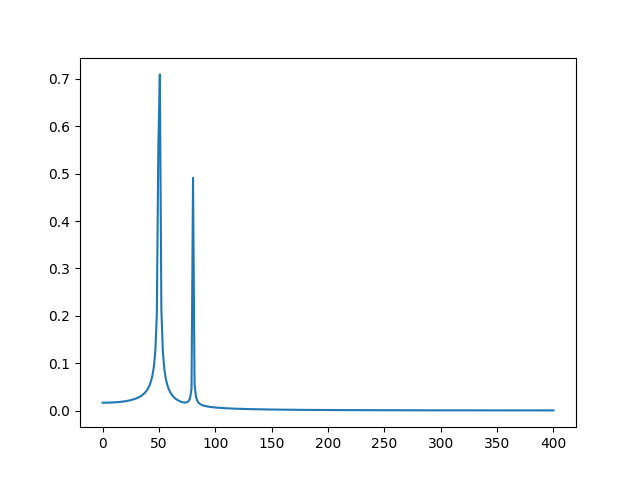
Signal processing
import scipy.signal as sc

# FIR filters - low pass, band stop
b1 = sc.firwin(40, 0.5)
b2 = sc.firwin(41, [0.3, 0.8])
w1, h1 = sc.freqz(b1)
w2, h2 = sc.freqz(b2)

plt.figure()
plt.title('Digital filter frequency response')
plt.plot(w1, 20*np.log10(np.abs(h1)), 'b', label='low pass')
plt.plot(w2, 20*np.log10(np.abs(h2)), 'r', label='band stop')
plt.ylabel('Amplitude Response (dB)')
plt.xlabel('Frequency (rad/sample)')
plt.legend()
plt.show()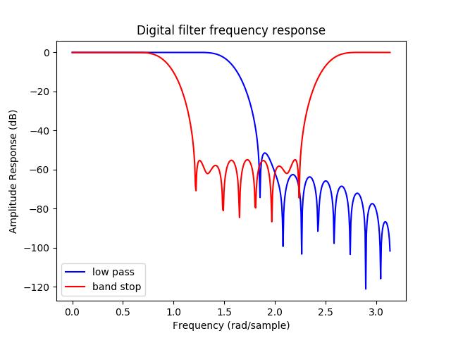
Linear algebra
import scipy.linalg as sc

# set of linear equations
A = np.array([[1, 2], [3, 4]])
b = np.array([[5], [6]])

# via inverse matrix
sc.inv(A).dot(b)

[[-4. ]
 [ 4.5]]

# via solver
sc.solve(A, b)

[[-4. ]
 [ 4.5]]
Statistics
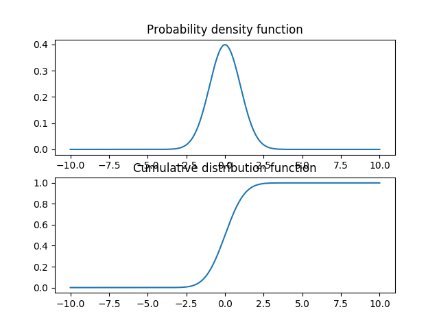
import scipy.stats as sc

# statistical parameters
x = sc.norm(size=100)
mean, std, var = x.mean(), x.std(), x.var()

(0.017051340606627, 0.97538562220022185, 0.95137711199491382)

# PDF, CDF
x = np.linspace(-10, 10, 1000)
y1 = sc.norm.pdf(x)
y2 = sc.norm.cdf(x)

plt.figure()
plt.subplot(211)
plt.plot(x, y1)
plt.title('Probability density function')
plt.subplot(212)
plt.plot(x, y2)
plt.title('Cumulative distribution function')
plt.show()